Chapter 4 Betting Strategy
Research3 shows the most successful betting strategy is the Kelly Criterion. The Kelly Criterion states that each bet should be equivalent to the percent edge. For example, with an expected value of 0.109, or a 10.9% edge, the bet should be equivalent to 10.9% of the bankroll. However, this strategy is contingent on having an extremely accurate model where the expected edge is the true edge. Due to limited data of just two seasons right now, many of the expected values are above 0.2, which would be a ludicrous amount of the bankroll to bet on one game. So, all expected values are capped at 0.2 with this method.
Starting with a bankroll of 100 units, the absolute maximum bet is capped at 40 because it became too easy to lose any sort of winnings while using the Kelly criterion.
Another system used modifications to the Kelly criterion system. In this system, the expected values essentially received a square root transformation; however, since the absolute value of the expected value must be less than one, this is actually a squared transformation. The new Kelly proportion is the expected value squared.
The Martingale betting system is another popular method. This betting system starts by betting a certain amount of units (in this case, 5 units). If the bet loses, the subsequent bet doubles, so that winning the bet leaves the bettor ahead by 5 units. If the second bet instead loses again, the third bet once again double – now to 20 units. This keeps on going until either the bankroll is empty or the bettor is ahead 5 units. This is a risky strategy.
One strategy simply bets 15 units any time there is a positive expected value. Another strategy only bets when there is an extreme edge; the bet is 10 units if the expected value is above 0.1 and 20 units if the expected values is above 0.2.
Finally, another betting system relied on the agreement of the two linear mixed models. If both models suggested betting on the same team, and each expected value is positive, then the system bets on this team. Betting amounts are determined with the Kelly Criterion, and the Kelly proportion is the average of the two different expected values generated from the different models.
The different betting systems are listed in Table 4.1.
| Strategy.Name | Description.of.Strategy |
|---|---|
| K1 | Kelly Criterion using team-specific stats mixed linear model. Best performing model by error. Max bet of 40 units. Capped expected value at 0.2. Utilize future betting strategy. |
| K2 | Kelly Criterion using betting-specific model. Max bet of 40 units. Capped expected value at 0.2. Utilize future betting strategy. |
| K3 | Kelly Criterion using simple linear regression model. Max bet of 40 units. Capped expected value at 0.2. Utilize future betting strategy. |
| K2 - Transform | Utilize same strategy as K1, but the Kelly proportion is the expected value squared. |
| Simple Bets | If positive expected value at first decision point from team-specific model, bet 15 units. If negative expected value, do not bet. Do not incorporate future betting strategy |
| Extreme Edge (Simple) | If edge at first decision point from team-specific model is greater than 0.1, bet 10 units. If greater than 0.2, bet 20 units. |
| Extreme Edge (Transform) | Only bet if the expected edge from team-specific model is greater than 0.1 and use Kelly Criterion with square transformation for betting amounts. Utilize future betting strategy. |
| Agreement | If both mixed linear models suggest betting on the same team, bet on that team. Use Kelly Criterion with a mean of the two expected values. Utilize future betting strategy. |
| Martingale | Use Martingale strategy if positive expected value from team-specific model. Use 5 units for initial bet. Do not incorporate future betting strategy. |
4.1 Results Using K-Fold Validation
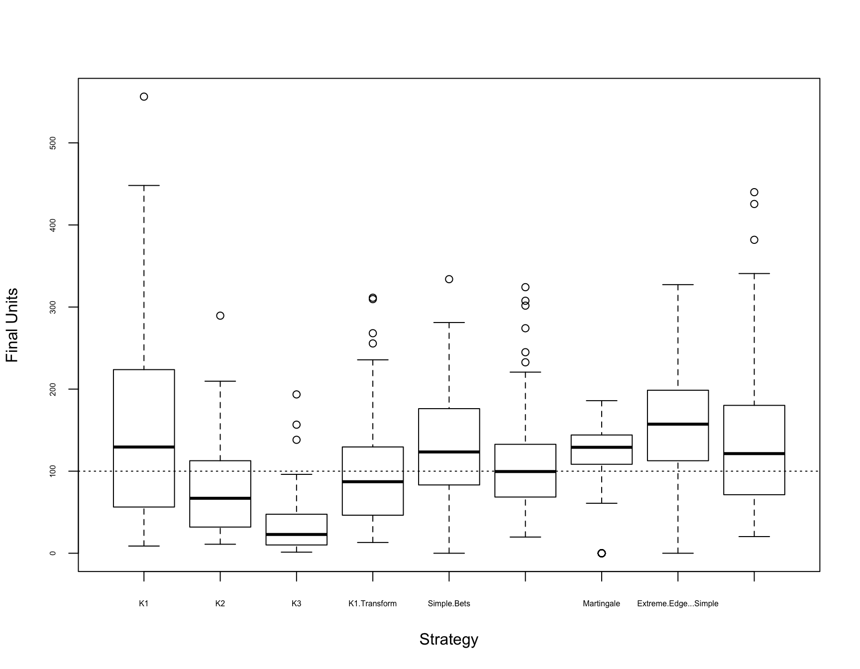
Figure 4.1: Final Bankroll Box Plots by Strategy
For each game in each test data set, the model went through the process outlined above for each betting strategy. After iterating through all the games in the test data set, I was left with the final bankroll from each model for each test data set in the k-fold. With 100 test data sets, I had a vector of 100 final bankrolls for each of the nine betting strategies.
Figure 4.1 is a boxplot looking at the distribution of the final bankrolls for each of the betting strategies over the 100 simulations. Most of the strategies have medians above 100, meaning they generated positive median returns. In addition, these distributions have a boundary on the low end of 0, as the strategy cannot end with a bankroll below 0, but with no maximum, the distributions tend to be right-skewed, leaving the means higher than the medians.
Table 4.2 shows the mean and median final bankrolls over the 100 simulations for the different methods. Four of the methods stand out; the K1 method, Martingale, Extreme Edge - Simple Bets and the LMER Agreement method. Outside of the Martingale method, which is interesting because this is the only strategy where the mean is significantly lower than the median, the other listed methods are noteworthy because of the huge returns – each of those three methods have mean returns above 35%.
| Mean Final Bankroll | Median Final Bankroll | |
|---|---|---|
| K1 | 153.61 | 129.42 |
| K2 | 80.88 | 66.99 |
| K3 | 33.55 | 22.89 |
| K1.Transform | 102.01 | 87.16 |
| Simple.Bets | 131.82 | 123.42 |
| Extreme.Edge…Transformed | 109.19 | 99.55 |
| Martingale | 113.62 | 129.09 |
| Extreme.Edge…Simple | 150.25 | 157.27 |
| LMER.Agreement | 137.62 | 121.40 |
Table 4.3 displays the summary statistics for the 4 top methods; the team-specific model using Kelly Criterion for betting amounts, the Martingale method, the Extreme Edge with Simple Bets and the Agreement method. The highest median is this K1 method. All these methods used the team-specific model to generate probabilities of beating the spread. The returns are very high in each of the quartiles, with positive returns for over 75% of simulations for the Extreme Edge with Simple Bets and Martingale methods. However, these are both the riskiest methods, as in 5% and 15%, respectively for each method, the bettor would have lost the entire bankroll using these methods. This is a very high chance relative to most other more standard investments in the stock market.
| Min. | 1st Qu. | Median | Mean | 3rd Qu. | Max. | |
|---|---|---|---|---|---|---|
| Kelly Criterion | 8.78 | 56.61 | 129.42 | 153.61 | 221.56 | 556.35 |
| Extreme Edge - Simple | 0.00 | 113.64 | 157.27 | 150.25 | 198.41 | 327.27 |
| Model Agreement | 20.31 | 71.41 | 121.40 | 137.62 | 179.07 | 439.94 |
| Martingale | 0.00 | 108.52 | 129.09 | 113.62 | 144.09 | 185.91 |
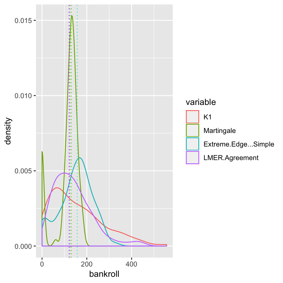
Figure 4.2: Density Plots comparing Four Successful Betting Strategies
Figure 4.2 shows the density plots for the 100 final bankrolls from the top four methods. The dotted lines represent the medians of each distribution. There seems to only be 3 dotted lines, but the medians for both the K1 and Martingale methods are both 129, so these lines are overlaid. The LMER-Agreement method seems to provide the safest betting strategy, as the density plot does not have as long of a tail, but a larger peak close to 175 units. It makes sense that this method is safest because this method only chooses to bet on games that both models agree on for whom to bet. Thus, a more selective group of games is chosen for bets. The Martingale method has 15% of observations at 0, but based on the nature of the bets, which continue to double if the bettor is losing, if the bettor does not lose the entire bankroll, it is a near guarantee to make money. The K1 and Extreme Edge - Simple methods both have extremely long tails and provide riskier investments than the LMER agreement methods, but also higher mean and median returns.
www.investopedia.com/articles/trading/04/091504.asp↩